Data processing

In this section you will find example of data processing.

Data is acquired in a RAW format from the TTM using the same data protocol for all the possible and different applications. Then depending on the type of information/application needed is unpacked, calibrated and reconstructed (Fig.1).

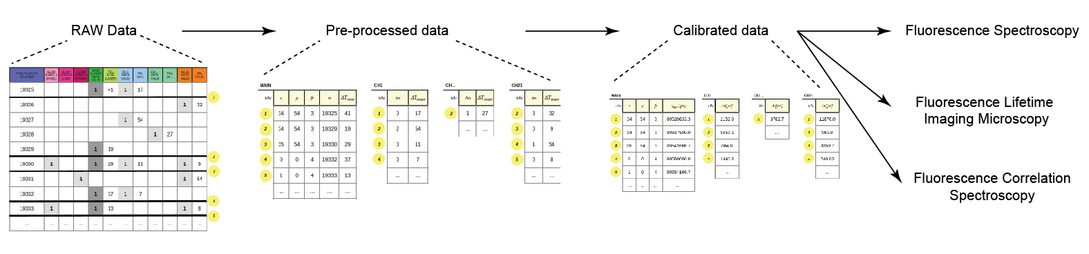
_images/DataProcessing.PNG — Fig.1 - Data processing procedure

In order to be able to reconstruct and process the data streamed by the BrightEyes-TTM python libraries have to be previously installed in the host-processing computer. On a normal desktop PC, the Jupyter Notebooks examples have from a couple of minutes up-to tenths of minutes of execution time.

Examples (firmware v2.0)

Before run the notebooks you need to install the libraries libttp and spadffs (v2.0)

libttp and spadffs (v2.0)

In order to read the raw data from the BrightEyes-TTM acquisition libttp is required. In the v2.0 you can easily install with the following command. Use an enviroment manager like venv

pip install libttp 

Moreover to run correctly the BrightEyes-TTM Notebook examples spadffs is needed too.

pip install -r https://raw.githubusercontent.com/VicidominiLab/libspadffs/ttm/requirements.txt
pip install git+https://github.com/VicidominiLab/libspadffs.git@ttm

(note you need to install "git" before run the last command, if you use a Conda enviroment use "conda install git")

Note

libttp uses Cython libraries. If you want to run in Windows you need to install Microsoft Build Tools. In Linux this is not required.

Notebooks

Before run the notebooks you need to install the libraries libttp and spadffs (v2.0)

TCSPC histogram

Thanks to the TCSPC histogram reconstruction Jupyter Notebook example it is possible to reconstruct and look the data from a simple spectroscopy point of view by building the TCSPC histogram for all the acquired channels.

Imaging

If pixel,line and frame clocks are connected to the BrightEyesTTM then intensity images as well as FLIM images can be reconstructed too. The image reconstruction Jupyter Notebook example shows all the steps to reconstruct a 4D dataset (x,y,t,ch) and visualize microscopy images.

FCS

If the final goal of the measurement is to retrieve information from the correlation curve the FCS Jupyter Notebook example shows how to calculate the correlation curve.

ISM & FLIM-Phasor analysis

This Jupyter notebook example can be used for implementing the pixel reassignment algorithm for image scanning microscopy (ISM) applications and for performing FLIM-phasor analysis with time-resolved data. After having used the image reconstruction Jupyter Notebook example for reconstructing a 4D dataset (x,y,t,ch) it is possible to feed this dataset into the ISM & FLIM-phasor notebook. NB - time alignment of the fluorescence lifetime decays is required, accross the different available channels (ch), before feeding a 4D dataset into this notebook.

Examples (legacy firmware v1.0)

Before run the notebooks you need to install the libraries libttp and spadffs (v1.0)

libttp and spadffs (legacy v1.0)

In order to install the libttp, spadffs version v1.0. Follow the links below for downloading and installing the required librares.

Note

libttp uses Cython libraries. If you want to run in Windows you need to install Microsoft Build Tools. In Linux this is not required.

TTM library for reconstructing and calibrating time-tagging data streamet by the BrightEyes-TTM to the host-PC - lipttp
FFS library for reconstructing the correlation curve and implementing FCS - spad_ffs

In order to give the user some preliminary tools to process, reconstruct and use the acquired TTM data we developed 3 main examples using Jupyter Notebook and we provide the associated examples dataset on Zenodo:

Notebooks

TCSPC histogram

Thanks to the TCSPC histogram reconstruction Jupyter Notebook example it is possible to reconstruct and look the data from a simple spectroscopy point of view by building the TCSPC histogram for all the acquired channels.

Imaging

If pixel,line and frame clocks are connected to the BrightEyesTTM then intensity images as well as FLIM images can be reconstructed too. The image reconstruction Jupyter Notebook example shows all the steps to reconstruct a 4D dataset (x,y,t,ch) and visualize microscopy images.

FCS

If the final goal of the measurement is to retrieve information from the correlation curve the FCS Jupyter Notebook example shows how to calculate the correlation curve.

ISM & FLIM-Phasor analysis

This Jupyter notebook example can be used for implementing the pixel reassignment algorithm for image scanning microscopy (ISM) applications and for performing FLIM-phasor analysis with time-resolved data. After having used the image reconstruction Jupyter Notebook example for reconstructing a 4D dataset (x,y,t,ch) it is possible to feed this dataset into the ISM & FLIM-phasor notebook. NB - time alignment of the fluorescence lifetime decays is required, accross the different available channels (ch), before feeding a 4D dataset into this notebook.

Data Source (Zenodo)

The data used in these examples can be downloaded from the link:

Name	Format	Associated example dataset on Zenodo
TSCPC Histogram	RAW legacy (v1.0)	Fluorescence_Spectroscopy_Dataset_40MHz
Imaging	RAW legacy (v1.0)	FLIM_512x512pixels_dwelltime250us_Dataset_40MHz
FCS	RAW legacy (v1.0)	FCS_scanfcs_Dataset_40MHz
TSCPC Histogram	RAW (v2.0)	FLIM_80MHz_512x512pixel_120FOV_pixeldwelltime200us.ttr
Imaging	RAW (v2.0)	FLIM_80MHz_512x512pixel_120FOV_pixeldwelltime200us.ttr
FCS	RAW (v2.0)	FCS_SpotVariation_80MHz.ttr